This is my first kaggle challenge. I needed help to complete it because I have only been studying deep learning and not data analysis. I did not know where to start or what to look for in doing data analysis. So I followed a previously done solution to the Titanic Challenge closely and tried to gain an intuition for everything that was done. This Jupyter notebook is that effort + the machine learning part in the end after the data analysis part!

from google.colab import drive
drive.mount('/content/drive')
Mounted at /content/drive
# Imports
import pandas as pd
import matplotlib.pyplot as plt
import numpy as np
I did a Kaggle Challenge and this is my work related to that. Everything above is my imports and connecting to my Google Drive for use in Google Colaboratory. Here is the Kaggle Challenge Link: https://www.kaggle.com/competitions/titanic/overview
Step 1: Explore the dataset and do data analysis.
Used https://www.kaggle.com/code/startupsci/titanic-data-science-solutions for data analysis inspiration
# Read in data and see a preview of it using .head()
data = pd.read_csv('./drive/MyDrive/Titanic_Challenge/train.csv')
data.head()
|
PassengerId |
Survived |
Pclass |
Name |
Sex |
Age |
SibSp |
Parch |
Ticket |
Fare |
Cabin |
Embarked |
| 0 |
1 |
0 |
3 |
Braund, Mr. Owen Harris |
male |
22.0 |
1 |
0 |
A/5 21171 |
7.2500 |
NaN |
S |
| 1 |
2 |
1 |
1 |
Cumings, Mrs. John Bradley (Florence Briggs Th... |
female |
38.0 |
1 |
0 |
PC 17599 |
71.2833 |
C85 |
C |
| 2 |
3 |
1 |
3 |
Heikkinen, Miss. Laina |
female |
26.0 |
0 |
0 |
STON/O2. 3101282 |
7.9250 |
NaN |
S |
| 3 |
4 |
1 |
1 |
Futrelle, Mrs. Jacques Heath (Lily May Peel) |
female |
35.0 |
1 |
0 |
113803 |
53.1000 |
C123 |
S |
| 4 |
5 |
0 |
3 |
Allen, Mr. William Henry |
male |
35.0 |
0 |
0 |
373450 |
8.0500 |
NaN |
S |
# Convert categorical datatypes 'Sex' and 'Embarked' into numeric
  # to do correlation calculation
numeric_df = data.select_dtypes(include=[float, int])
numeric_df['Sex'] = data['Sex'].map({'male': 0, 'female':1})
numeric_df['Embarked'] = data['Embarked'].map({'S':0, 'C':1, 'Q':2})

# numeric_df.head()
numeric_df.corr()
|
PassengerId |
Survived |
Pclass |
Age |
SibSp |
Parch |
Fare |
Sex |
Embarked |
| PassengerId |
1.000000 |
-0.005007 |
-0.035144 |
0.036847 |
-0.057527 |
-0.001652 |
0.012658 |
-0.042939 |
-0.030555 |
| Survived |
-0.005007 |
1.000000 |
-0.338481 |
-0.077221 |
-0.035322 |
0.081629 |
0.257307 |
0.543351 |
0.108669 |
| Pclass |
-0.035144 |
-0.338481 |
1.000000 |
-0.369226 |
0.083081 |
0.018443 |
-0.549500 |
-0.131900 |
0.043835 |
| Age |
0.036847 |
-0.077221 |
-0.369226 |
1.000000 |
-0.308247 |
-0.189119 |
0.096067 |
-0.093254 |
0.012186 |
| SibSp |
-0.057527 |
-0.035322 |
0.083081 |
-0.308247 |
1.000000 |
0.414838 |
0.159651 |
0.114631 |
-0.060606 |
| Parch |
-0.001652 |
0.081629 |
0.018443 |
-0.189119 |
0.414838 |
1.000000 |
0.216225 |
0.245489 |
-0.079320 |
| Fare |
0.012658 |
0.257307 |
-0.549500 |
0.096067 |
0.159651 |
0.216225 |
1.000000 |
0.182333 |
0.063462 |
| Sex |
-0.042939 |
0.543351 |
-0.131900 |
-0.093254 |
0.114631 |
0.245489 |
0.182333 |
1.000000 |
0.118593 |
| Embarked |
-0.030555 |
0.108669 |
0.043835 |
0.012186 |
-0.060606 |
-0.079320 |
0.063462 |
0.118593 |
1.000000 |
Gain an intuition for how the correlation calculation works by using a tiny example. What I found: the best correlations have graphs that depict a monotonic relationship like the sigmoid function and not snake curves like the piece wise function (graphed below)
# Prove to myself that outputs going up and down will give a bad correlation
# Correlation only captures monotonic relationships
import numpy as np
import matplotlib.pyplot as plt
import pandas as pd

def piecewise(x):
    if x < -5:
        return 0
    elif -5 <= x < 0:
        return 1
    elif 0 <= x < 5:
        return 0
    else:
        return 1

# Generate x values
x = np.linspace(-10, 10, 400)  # 400 points from -10 to 10

# Apply the piecewise function to each x value
y = np.array([piecewise(xi) for xi in x])

# Plotting the Sigmoid function
plt.figure(figsize=(10, 6))
plt.plot(x, y, label='Piecewise Function')
plt.title('Piecewise Function')
plt.xlabel('X values')
plt.ylabel('Piecewise Output')
plt.grid(True)
plt.legend()
plt.show()

# Create a DataFrame
data_piecewise = pd.DataFrame({'X': x, 'Y': y})

# Calculate correlation
correlation = data_piecewise['X'].corr(data_piecewise['Y'])
print("Correlation coefficient:", correlation)

# Monotonic function - Sigmoid function
def sigmoid(x):
    return 1 / (1 + np.exp(-x))

# Apply the sigmoid function to each x value
y_sigmoid = np.array([sigmoid(xi) for xi in x])

# Plotting the Sigmoid function on the same plot
plt.plot(x, y_sigmoid, label='Sigmoid Function', linestyle='--')
plt.legend()
plt.show()

# Create a DataFrame for the sigmoid function
data_sigmoid = pd.DataFrame({'X': x, 'Y_Sigmoid': y_sigmoid})

# Calculate correlation for sigmoid
correlation_sigmoid = data_sigmoid['X'].corr(data_sigmoid['Y_Sigmoid'])
print("Sigmoid Correlation coefficient:", correlation_sigmoid)
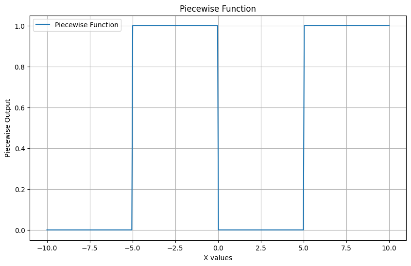
Correlation coefficient: 0.43301405506325596
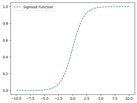
Sigmoid Correlation coefficient: 0.9362677445388511
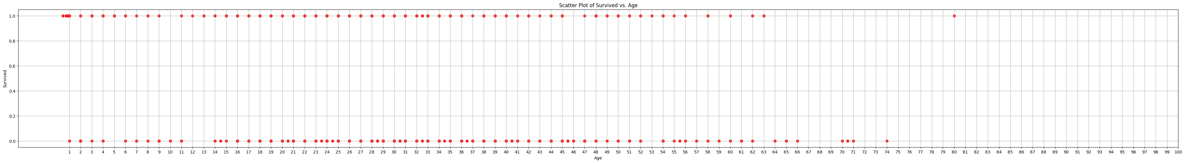
Below plot shows why pandas.corr() may not be the most reliable metric for showing which features(Age, Embarked,etc) are the most important to deciding whether a passenger lived or died. The data is up and down: As age goes up there is no clear rise or fall in deaths its behaving more like the piece wise function and not like the sigmoid function above.
# Completely useless plot
# But it shows why the correlation calculation would not work.
# The data is up and down like the piece wise function above
plt.figure(figsize=(50,6))
plt.scatter(data['Age'], data['Survived'], alpha=1, color='red')
plt.title("Scatter Plot of Survived vs. Age")
plt.xlabel('Age')
plt.ylabel('Survived')
plt.xticks(range(1, 101, 1))
plt.grid(True)
plt.show()
# Determine Age bands and check correlation with Survived
# print(pd.cut(data['Age'],5))
# print(data['Age'].head())
data['AgeBand'] = pd.cut(data['Age'], 5)
data[['AgeBand','Survived']].groupby(['AgeBand'], as_index=False).mean().sort_values(by='AgeBand', ascending=True)
|
AgeBand |
Survived |
| 0 |
(0.34, 16.336] |
0.550000 |
| 1 |
(16.336, 32.252] |
0.369942 |
| 2 |
(32.252, 48.168] |
0.404255 |
| 3 |
(48.168, 64.084] |
0.434783 |
| 4 |
(64.084, 80.0] |
0.090909 |
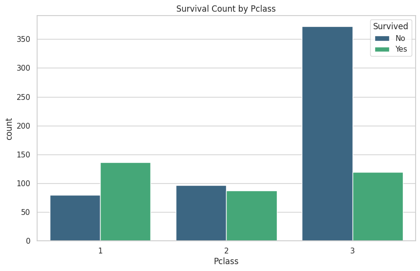
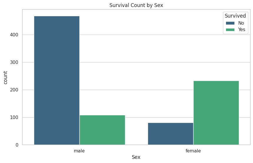
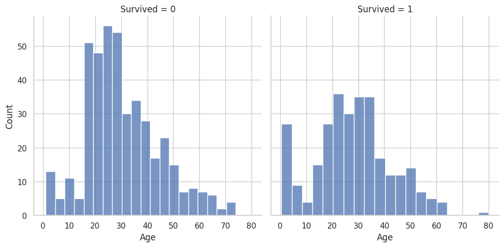
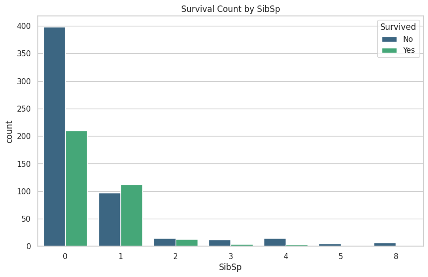
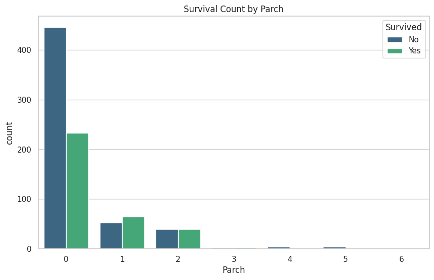
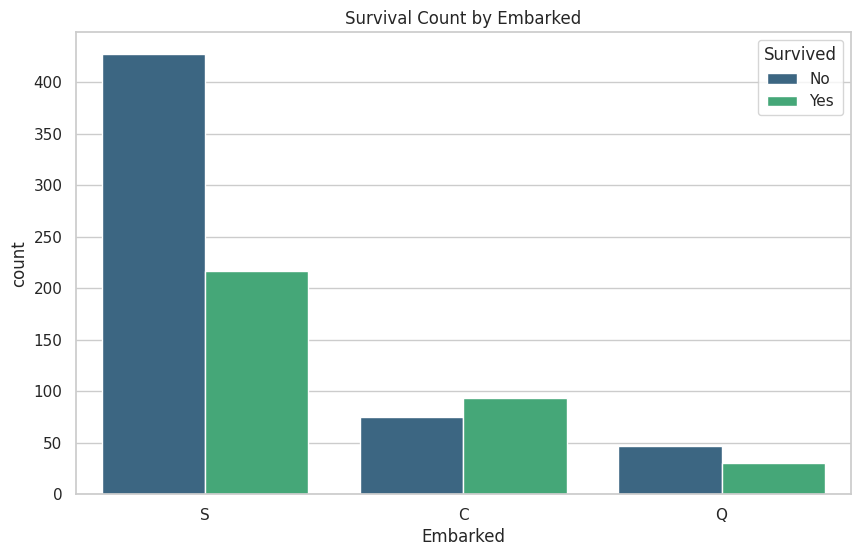
These are the graphs that I mainly relied on for my analysis because it shows the correlation between deaths and the other classes well. “Oh look the lower class people tended to not be survivors”
# These graphs are gold!
# Load and analyze the data
import matplotlib.pyplot as plt
import seaborn as sns
# Set the style for the plots
sns.set(style="whitegrid")
# Columns to plot, excluding 'PassengerId', 'Name', 'Ticket', 'Cabin' due to their specificity or lack of relevance
columns_to_plot = ['Pclass', 'Sex', 'Age', 'SibSp', 'Parch', 'Fare', 'Embarked']
# Define a function to plot survival count based on a given feature
def plot_survival(data, column):
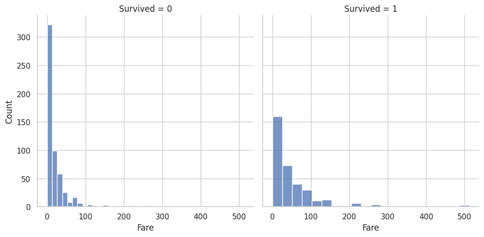
if column=='Age' or column=='Fare':
g = sns.FacetGrid(data, col='Survived', height=5, aspect=1)
g.map(sns.histplot, column, bins=20, kde=False)
else:
# Create a count plot for categorical data
plt.figure(figsize=(10, 6))
sns.countplot(x=column, hue='Survived', data=data, palette='viridis')
plt.title(f'Survival Count by {column}')
plt.legend(title='Survived', loc='upper right', labels=['No', 'Yes'])
plt.show()
# Create a loop to generate plots for each relevant column
for column in columns_to_plot:
plot_survival(data, column)
# Read in training and test dataset
# Previous analysis above was also on training dataset it just had a different variable name
# Now calling training dataset train_df
train_df = pd.read_csv('./drive/MyDrive/Titanic_Challenge/train.csv')
test_df = pd.read_csv('./drive/MyDrive/Titanic_Challenge/test.csv')
# Get info on the train vs. test datasets
train_df.info()
print('_'*40)
test_df.info()
<class 'pandas.core.frame.DataFrame'>
RangeIndex: 891 entries, 0 to 890
Data columns (total 12 columns):
 #   Column       Non-Null Count  Dtype
---  ------       --------------  -----
 0   PassengerId  891 non-null    int64
 1   Survived     891 non-null    int64
 2   Pclass       891 non-null    int64
 3   Name         891 non-null    object
 4   Sex          891 non-null    object
 5   Age          714 non-null    float64
 6   SibSp        891 non-null    int64
 7   Parch        891 non-null    int64
 8   Ticket       891 non-null    object
 9   Fare         891 non-null    float64
 10  Cabin        204 non-null    object
 11  Embarked     889 non-null    object
dtypes: float64(2), int64(5), object(5)
memory usage: 83.7+ KB
________________________________________
<class 'pandas.core.frame.DataFrame'>
RangeIndex: 418 entries, 0 to 417
Data columns (total 11 columns):
 #   Column       Non-Null Count  Dtype
---  ------       --------------  -----
 0   PassengerId  418 non-null    int64
 1   Pclass       418 non-null    int64
 2   Name         418 non-null    object
 3   Sex          418 non-null    object
 4   Age          332 non-null    float64
 5   SibSp        418 non-null    int64
 6   Parch        418 non-null    int64
 7   Ticket       418 non-null    object
 8   Fare         417 non-null    float64
 9   Cabin        91 non-null     object
 10  Embarked     418 non-null    object
dtypes: float64(2), int64(4), object(5)
memory usage: 36.0+ KB
# Get statistics on the numerical categories in the dataset like Age and PClass(1,2,3)
train_df.describe()
|
PassengerId |
Survived |
Pclass |
Age |
SibSp |
Parch |
Fare |
| count |
891.000000 |
891.000000 |
891.000000 |
714.000000 |
891.000000 |
891.000000 |
891.000000 |
| mean |
446.000000 |
0.383838 |
2.308642 |
29.699118 |
0.523008 |
0.381594 |
32.204208 |
| std |
257.353842 |
0.486592 |
0.836071 |
14.526497 |
1.102743 |
0.806057 |
49.693429 |
| min |
1.000000 |
0.000000 |
1.000000 |
0.420000 |
0.000000 |
0.000000 |
0.000000 |
| 25% |
223.500000 |
0.000000 |
2.000000 |
20.125000 |
0.000000 |
0.000000 |
7.910400 |
| 50% |
446.000000 |
0.000000 |
3.000000 |
28.000000 |
0.000000 |
0.000000 |
14.454200 |
| 75% |
668.500000 |
1.000000 |
3.000000 |
38.000000 |
1.000000 |
0.000000 |
31.000000 |
| max |
891.000000 |
1.000000 |
3.000000 |
80.000000 |
8.000000 |
6.000000 |
512.329200 |
# Describe categorical data
# the include=['O'] means to include types that are objects
train_df.describe(include='O')
|
Name |
Sex |
Ticket |
Cabin |
Embarked |
| count |
891 |
891 |
891 |
204 |
889 |
| unique |
891 |
2 |
681 |
147 |
3 |
| top |
Braund, Mr. Owen Harris |
male |
347082 |
B96 B98 |
S |
| freq |
1 |
577 |
7 |
4 |
644 |
Mean statistics of each class. Mean Calculation is:
total of survived(survived = 1) / total(survived=0 + survived=1)
# P class vs Survived Mean Stat
# Mean stat is where we get the mean of the values for each category in PClass that survived
# This gives the mean of each PClass that survived.
# Look at Class 3!!!
train_df[['Pclass', 'Survived']].groupby(['Pclass'], as_index=False).mean().sort_values(by='Survived', ascending=False)
|
Pclass |
Survived |
| 0 |
1 |
0.629630 |
| 1 |
2 |
0.472826 |
| 2 |
3 |
0.242363 |
train_df[['Sex', 'Survived']].groupby(['Sex'], as_index=False).mean().sort_values(by='Survived', ascending=False)
# Females were more likely to survive than males
|
Sex |
Survived |
| 0 |
female |
0.742038 |
| 1 |
male |
0.188908 |
train_df[['Embarked', 'Survived']].groupby(['Embarked'], as_index=False).mean().sort_values(by='Survived', ascending=False)
# The station people left from might be correlated with their PClass
|
Embarked |
Survived |
| 0 |
C |
0.553571 |
| 1 |
Q |
0.389610 |
| 2 |
S |
0.336957 |
# Number of Parents+Children => Parch
train_df[['Parch', 'Survived']].groupby(['Parch'], as_index=False).mean().sort_values(by='Parch', ascending=True)
|
Parch |
Survived |
| 0 |
0 |
0.343658 |
| 1 |
1 |
0.550847 |
| 2 |
2 |
0.500000 |
| 3 |
3 |
0.600000 |
| 4 |
4 |
0.000000 |
| 5 |
5 |
0.200000 |
| 6 |
6 |
0.000000 |
# Sibsp => Number of siblings + Spouse
train_df[['SibSp', 'Survived']].groupby(['SibSp'], as_index=False).mean().sort_values(by='SibSp', ascending=True)
|
SibSp |
Survived |
| 0 |
0 |
0.345395 |
| 1 |
1 |
0.535885 |
| 2 |
2 |
0.464286 |
| 3 |
3 |
0.250000 |
| 4 |
4 |
0.166667 |
| 5 |
5 |
0.000000 |
| 6 |
8 |
0.000000 |
train_df[['SibSp', 'Pclass']].groupby(['SibSp', 'Pclass'], as_index=False).value_counts()
|
SibSp |
Pclass |
count |
| 0 |
0 |
1 |
137 |
| 1 |
0 |
2 |
120 |
| 2 |
0 |
3 |
351 |
| 3 |
1 |
1 |
71 |
| 4 |
1 |
2 |
55 |
| 5 |
1 |
3 |
83 |
| 6 |
2 |
1 |
5 |
| 7 |
2 |
2 |
8 |
| 8 |
2 |
3 |
15 |
| 9 |
3 |
1 |
3 |
| 10 |
3 |
2 |
1 |
| 11 |
3 |
3 |
12 |
| 12 |
4 |
3 |
18 |
| 13 |
5 |
3 |
5 |
| 14 |
8 |
3 |
7 |
train_df[['Parch', 'Pclass']].groupby(['Parch', 'Pclass'], as_index=False).value_counts()
|
Parch |
Pclass |
count |
| 0 |
0 |
1 |
163 |
| 1 |
0 |
2 |
134 |
| 2 |
0 |
3 |
381 |
| 3 |
1 |
1 |
31 |
| 4 |
1 |
2 |
32 |
| 5 |
1 |
3 |
55 |
| 6 |
2 |
1 |
21 |
| 7 |
2 |
2 |
16 |
| 8 |
2 |
3 |
43 |
| 9 |
3 |
2 |
2 |
| 10 |
3 |
3 |
3 |
| 11 |
4 |
1 |
1 |
| 12 |
4 |
3 |
3 |
| 13 |
5 |
3 |
5 |
| 14 |
6 |
3 |
1 |
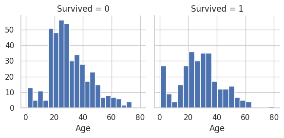
Clearer view graphs. To get a clearer view of who survived vs. who did not for specific classes we are interested in
# Get a clear view of Age range and who did not survive (0) vs. who survived (1)
g = sns.FacetGrid(train_df, col='Survived')
g.map(plt.hist, 'Age', bins=20)
<seaborn.axisgrid.FacetGrid at 0x7fbc33717490>
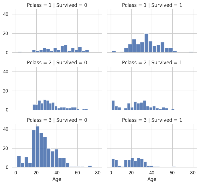
# Age range and P Class for who did not survive(0) vs. who survived(1)
grid = sns.FacetGrid(train_df, col='Survived', row='Pclass', height=2.2, aspect=1.6)
grid.map(plt.hist, 'Age', alpha=0.9, bins=20)
grid.add_legend();
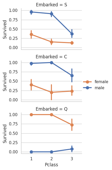
# Station embarked, male/female, and P Class for who did not survive vs who survived
# As you can see the male survival rate is higher for the first two stations
# But then there is a higer survival rate
# The survival rate always drops off for lower PClass
  # (Except in station C for female PClass 3)
grid = sns.FacetGrid(train_df, row='Embarked', height=2.2, aspect=1.6)
grid.map(sns.pointplot, 'Pclass', 'Survived', 'Sex', palette='deep')
grid.add_legend()
/usr/local/lib/python3.10/dist-packages/seaborn/axisgrid.py:718: UserWarning: Using the pointplot function without specifying `order` is likely to produce an incorrect plot.
  warnings.warn(warning)
/usr/local/lib/python3.10/dist-packages/seaborn/axisgrid.py:723: UserWarning: Using the pointplot function without specifying `hue_order` is likely to produce an incorrect plot.
  warnings.warn(warning)


<seaborn.axisgrid.FacetGrid at 0x7fbc3343a7d0>
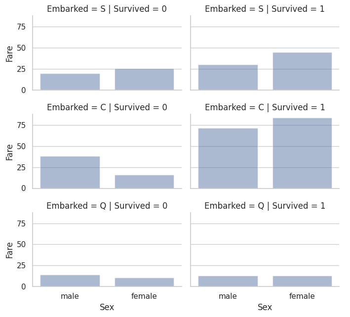
# Different embarked stations and male vs. female at those stations
  # Survived vs did not survive
grid = sns.FacetGrid(train_df, row='Embarked', col='Survived', height=2.2, aspect=1.6)
grid.map(sns.barplot, 'Sex', 'Fare', alpha=.5, errorbar=None)
grid.add_legend()
/usr/local/lib/python3.10/dist-packages/seaborn/axisgrid.py:718: UserWarning: Using the barplot function without specifying `order` is likely to produce an incorrect plot.
  warnings.warn(warning)


<seaborn.axisgrid.FacetGrid at 0x7fbc3384d000>
- by dropping features that will not have correlation to survival. Like ticket number and cabin
- And transforming categorical features like embarked station to numerical feature because the ML algorithms do not understand categorical features.
- Also creating new features out of the existing features that may be helpful. Like extracting titles from names.
- Filling in null values since some ML classifiers cannot handle null.
# Correcting by dropping features
# Drop ticket and cabin number features
combine = [train_df, test_df]
print("Before", train_df.shape, test_df.shape, combine[0].shape, combine[1].shape)

train_df = train_df.drop(['Ticket', 'Cabin'], axis=1)
test_df = test_df.drop(['Ticket', 'Cabin'], axis=1)
combine = [train_df, test_df]

"After", train_df.shape, test_df.shape, combine[0].shape, combine[1].shape
Before (891, 12) (418, 11) (891, 12) (418, 11)


('After', (891, 10), (418, 9), (891, 10), (418, 9))
The blog I am following talks about creating a new feature out of the name feature called titles. Because it may have some correlation to who survived and who did not.
# Create title feature
for dataset in combine:
    dataset['Title'] = dataset.Name.str.extract(' ([A-Za-z]+)\.', expand=False)

pd.crosstab(train_df['Title'], train_df['Sex'])
| Sex |
female |
male |
| Title |
|
|
| Capt |
0 |
1 |
| Col |
0 |
2 |
| Countess |
1 |
0 |
| Don |
0 |
1 |
| Dr |
1 |
6 |
| Jonkheer |
0 |
1 |
| Lady |
1 |
0 |
| Major |
0 |
2 |
| Master |
0 |
40 |
| Miss |
182 |
0 |
| Mlle |
2 |
0 |
| Mme |
1 |
0 |
| Mr |
0 |
517 |
| Mrs |
125 |
0 |
| Ms |
1 |
0 |
| Rev |
0 |
6 |
| Sir |
0 |
1 |
# Mean statistic on survival with new title feature
for dataset in combine:
    dataset['Title'] = dataset['Title'].replace(['Lady', 'Countess','Capt', 'Col',\
 	'Don', 'Dr', 'Major', 'Rev', 'Sir', 'Jonkheer', 'Dona'], 'Rare')

    dataset['Title'] = dataset['Title'].replace('Mlle', 'Miss')
    dataset['Title'] = dataset['Title'].replace('Ms', 'Miss')
    dataset['Title'] = dataset['Title'].replace('Mme', 'Mrs')

train_df[['Title', 'Survived']].groupby(['Title'], as_index=False).mean().sort_values('Survived')
|
Title |
Survived |
| 2 |
Mr |
0.156673 |
| 4 |
Rare |
0.347826 |
| 0 |
Master |
0.575000 |
| 1 |
Miss |
0.702703 |
| 3 |
Mrs |
0.793651 |
# Transfer the rarer titles to a overall Rare category
title_mapping = {"Mr": 1, "Miss": 2, "Mrs": 3, "Master": 4, "Rare": 5}
for dataset in combine:
    dataset['Title'] = dataset['Title'].map(title_mapping)
    dataset['Title'] = dataset['Title'].fillna(0)

# See transformed dataset
train_df.head()
|
PassengerId |
Survived |
Pclass |
Name |
Sex |
Age |
SibSp |
Parch |
Fare |
Embarked |
Title |
| 0 |
1 |
0 |
3 |
Braund, Mr. Owen Harris |
male |
22.0 |
1 |
0 |
7.2500 |
S |
1 |
| 1 |
2 |
1 |
1 |
Cumings, Mrs. John Bradley (Florence Briggs Th... |
female |
38.0 |
1 |
0 |
71.2833 |
C |
3 |
| 2 |
3 |
1 |
3 |
Heikkinen, Miss. Laina |
female |
26.0 |
0 |
0 |
7.9250 |
S |
2 |
| 3 |
4 |
1 |
1 |
Futrelle, Mrs. Jacques Heath (Lily May Peel) |
female |
35.0 |
1 |
0 |
53.1000 |
S |
3 |
| 4 |
5 |
0 |
3 |
Allen, Mr. William Henry |
male |
35.0 |
0 |
0 |
8.0500 |
S |
1 |
# Drop name and PassengerId features for test and training datasets
train_df = train_df.drop(['Name', 'PassengerId'], axis=1)
test_df = test_df.drop(['Name'], axis=1)
combine = [train_df, test_df]
train_df.shape, test_df.shape
# Convert categorical sex feature (male, female) to numeric feature
for dataset in combine:
    dataset['Sex'] = dataset['Sex'].map( {'female': 1, 'male': 0} ).astype(int)

train_df.head()
|
Survived |
Pclass |
Sex |
Age |
SibSp |
Parch |
Fare |
Embarked |
Title |
| 0 |
0 |
3 |
0 |
22.0 |
1 |
0 |
7.2500 |
S |
1 |
| 1 |
1 |
1 |
1 |
38.0 |
1 |
0 |
71.2833 |
C |
3 |
| 2 |
1 |
3 |
1 |
26.0 |
0 |
0 |
7.9250 |
S |
2 |
| 3 |
1 |
1 |
1 |
35.0 |
1 |
0 |
53.1000 |
S |
3 |
| 4 |
0 |
3 |
0 |
35.0 |
0 |
0 |
8.0500 |
S |
1 |
# Completing values for missing or null values
# For which columns?
# Age
print(len(train_df['Age']))
train_df['Age'].unique()
print(train_df['Age'].isna().sum())
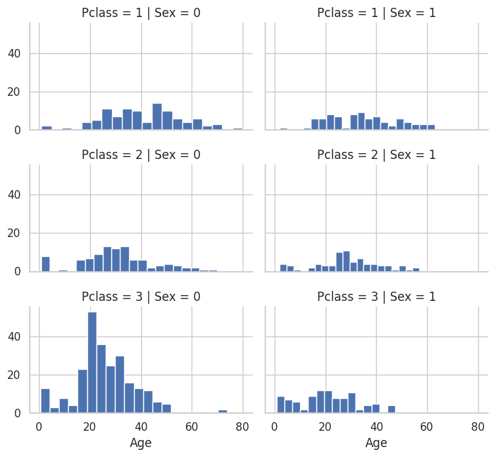
# More accurate way of guessing missing values is to use other correlated features.
# In our case we note correlation among Age, Gender, and Pclass.
# Guess Age values using median values for Age across sets of Pclass and Gender feature combinations.
# So, median Age for Pclass=1 and Gender=0, Pclass=1 and Gender=1, and so on..
grid = sns.FacetGrid(train_df, row='Pclass', col='Sex', height=2.2, aspect=1.6)
grid.map(plt.hist, 'Age', alpha=1, bins=20)
grid.add_legend()
891
177


<seaborn.axisgrid.FacetGrid at 0x7fbc330248b0>
# Guessed values of Age for different combinations of Pclass and Sex
# Fill in the guessed age values where age is null

guess_ages = np.zeros((2,3))
# Iterate over Sex (0,1) and Pclass(1,2,3) to calculate guessed values of Age for the six combinations
for dataset in combine:
    for i in range(0, 2):
        for j in range(0, 3):
            guess_df = dataset[(dataset['Sex'] == i) & \
                                  (dataset['Pclass'] == j+1)]['Age'].dropna()

            # age_mean = guess_df.mean()
            # age_std = guess_df.std()
            # age_guess = rnd.uniform(age_mean - age_std, age_mean + age_std)

            age_guess = guess_df.median()

            # Convert random age float to nearest .5 age
            guess_ages[i,j] = int( age_guess/0.5 + 0.5 ) * 0.5

    # Fill in the guessed age values where age is null in the dataset
    for i in range(0, 2):
        for j in range(0, 3):
            dataset.loc[ (dataset.Age.isnull()) & (dataset.Sex == i) & (dataset.Pclass == j+1),\
                    'Age'] = guess_ages[i,j]

    dataset['Age'] = dataset['Age'].astype(int)

train_df.head()
|
Survived |
Pclass |
Sex |
Age |
SibSp |
Parch |
Fare |
Embarked |
Title |
| 0 |
0 |
3 |
0 |
22 |
1 |
0 |
7.2500 |
S |
1 |
| 1 |
1 |
1 |
1 |
38 |
1 |
0 |
71.2833 |
C |
3 |
| 2 |
1 |
3 |
1 |
26 |
0 |
0 |
7.9250 |
S |
2 |
| 3 |
1 |
1 |
1 |
35 |
1 |
0 |
53.1000 |
S |
3 |
| 4 |
0 |
3 |
0 |
35 |
0 |
0 |
8.0500 |
S |
1 |
# Create Age Bands and determine correlations with Survived
train_df['AgeBand'] = pd.cut(train_df['Age'], 5)
train_df[['AgeBand', 'Survived']].groupby(['AgeBand'], as_index=False).mean().sort_values(by='AgeBand', ascending=True)
|
AgeBand |
Survived |
| 0 |
(-0.08, 16.0] |
0.550000 |
| 1 |
(16.0, 32.0] |
0.337374 |
| 2 |
(32.0, 48.0] |
0.412037 |
| 3 |
(48.0, 64.0] |
0.434783 |
| 4 |
(64.0, 80.0] |
0.090909 |
# Replace age with ordinals for these bands
for dataset in combine:
    dataset.loc[ dataset['Age'] <= 16, 'Age'] = 0
    dataset.loc[(dataset['Age'] > 16) & (dataset['Age'] <= 32), 'Age'] = 1
    dataset.loc[(dataset['Age'] > 32) & (dataset['Age'] <= 48), 'Age'] = 2
    dataset.loc[(dataset['Age'] > 48) & (dataset['Age'] <= 64), 'Age'] = 3
    dataset.loc[ dataset['Age'] > 64, 'Age']
train_df.head()
|
Survived |
Pclass |
Sex |
Age |
SibSp |
Parch |
Fare |
Embarked |
Title |
AgeBand |
| 0 |
0 |
3 |
0 |
1 |
1 |
0 |
7.2500 |
S |
1 |
(16.0, 32.0] |
| 1 |
1 |
1 |
1 |
2 |
1 |
0 |
71.2833 |
C |
3 |
(32.0, 48.0] |
| 2 |
1 |
3 |
1 |
1 |
0 |
0 |
7.9250 |
S |
2 |
(16.0, 32.0] |
| 3 |
1 |
1 |
1 |
2 |
1 |
0 |
53.1000 |
S |
3 |
(32.0, 48.0] |
| 4 |
0 |
3 |
0 |
2 |
0 |
0 |
8.0500 |
S |
1 |
(32.0, 48.0] |
# Remove the age band feature
train_df = train_df.drop(['AgeBand'], axis=1)
combine = [train_df, test_df]
train_df.head()
|
Survived |
Pclass |
Sex |
Age |
SibSp |
Parch |
Fare |
Embarked |
Title |
| 0 |
0 |
3 |
0 |
1 |
1 |
0 |
7.2500 |
S |
1 |
| 1 |
1 |
1 |
1 |
2 |
1 |
0 |
71.2833 |
C |
3 |
| 2 |
1 |
3 |
1 |
1 |
0 |
0 |
7.9250 |
S |
2 |
| 3 |
1 |
1 |
1 |
2 |
1 |
0 |
53.1000 |
S |
3 |
| 4 |
0 |
3 |
0 |
2 |
0 |
0 |
8.0500 |
S |
1 |
# Create a new feature called 'FamilySize' which combines Parch and SibSp.
# This will enable us to drop Parch and SibSp from the datasets
for dataset in combine:
    # We are adding 1 to count ourselves as a person
    dataset['FamilySize'] = dataset['SibSp'] + dataset['Parch'] + 1

train_df[['FamilySize', 'Survived']].groupby(['FamilySize'], as_index=False).mean().sort_values(by='Survived', ascending=False)
|
FamilySize |
Survived |
| 3 |
4 |
0.724138 |
| 2 |
3 |
0.578431 |
| 1 |
2 |
0.552795 |
| 6 |
7 |
0.333333 |
| 0 |
1 |
0.303538 |
| 4 |
5 |
0.200000 |
| 5 |
6 |
0.136364 |
| 7 |
8 |
0.000000 |
| 8 |
11 |
0.000000 |
# Calculate statistics for people that survived who were alone
# Vs. ones that had family
for dataset in combine:
    dataset['IsAlone'] = 0
    dataset.loc[dataset['FamilySize'] == 1, 'IsAlone'] = 1

train_df[['IsAlone', 'Survived']].groupby(['IsAlone'], as_index=False).mean()
|
IsAlone |
Survived |
| 0 |
0 |
0.505650 |
| 1 |
1 |
0.303538 |
# Find the most frequently occurring port
freq_port = train_df.Embarked.dropna().mode()[0]
freq_port
# Fill missing port values with the most frequent occurring port
for dataset in combine:
    dataset['Embarked'] = dataset['Embarked'].fillna(freq_port)

train_df[['Embarked', 'Survived']].groupby(['Embarked'], as_index=False).mean().sort_values(by='Survived', ascending=False)
|
Embarked |
Survived |
| 0 |
C |
0.553571 |
| 1 |
Q |
0.389610 |
| 2 |
S |
0.339009 |
# Convert categorical port to numeric port feature
for dataset in combine:
    dataset['Embarked'] = dataset['Embarked'].map( {'S': 0, 'C': 1, 'Q': 2} ).astype(int)

train_df.head()
|
Survived |
Pclass |
Sex |
Age |
SibSp |
Parch |
Fare |
Embarked |
Title |
FamilySize |
IsAlone |
| 0 |
0 |
3 |
0 |
1 |
1 |
0 |
7.2500 |
0 |
1 |
2 |
0 |
| 1 |
1 |
1 |
1 |
2 |
1 |
0 |
71.2833 |
1 |
3 |
2 |
0 |
| 2 |
1 |
3 |
1 |
1 |
0 |
0 |
7.9250 |
0 |
2 |
1 |
1 |
| 3 |
1 |
1 |
1 |
2 |
1 |
0 |
53.1000 |
0 |
3 |
2 |
0 |
| 4 |
0 |
3 |
0 |
2 |
0 |
0 |
8.0500 |
0 |
1 |
1 |
1 |
# The test data set had a single missing value for fare so we are filling that in
# The model algorithm needs to operate on nonnull values
# Round off the fare to two decimals because it represents currency
test_df['Fare'].fillna(test_df['Fare'].dropna().median(), inplace=True)
test_df.head()
|
PassengerId |
Pclass |
Sex |
Age |
SibSp |
Parch |
Fare |
Embarked |
Title |
FamilySize |
IsAlone |
| 0 |
892 |
3 |
0 |
2 |
0 |
0 |
7.8292 |
2 |
1 |
1 |
1 |
| 1 |
893 |
3 |
1 |
2 |
1 |
0 |
7.0000 |
0 |
3 |
2 |
0 |
| 2 |
894 |
2 |
0 |
3 |
0 |
0 |
9.6875 |
2 |
1 |
1 |
1 |
| 3 |
895 |
3 |
0 |
1 |
0 |
0 |
8.6625 |
0 |
1 |
1 |
1 |
| 4 |
896 |
3 |
1 |
1 |
1 |
1 |
12.2875 |
0 |
3 |
3 |
0 |
# Fareband and survived mean stat

train_df['FareBand'] = pd.qcut(train_df['Fare'], 4)
train_df[['FareBand', 'Survived']].groupby(['FareBand'], as_index=False).mean().sort_values(by='FareBand', ascending=True)
|
FareBand |
Survived |
| 0 |
(-0.001, 7.91] |
0.197309 |
| 1 |
(7.91, 14.454] |
0.303571 |
| 2 |
(14.454, 31.0] |
0.454955 |
| 3 |
(31.0, 512.329] |
0.581081 |
# Convert the Fare Feature to ordinal values based on FareBand
for dataset in combine:
    dataset.loc[ dataset['Fare'] <= 7.91, 'Fare'] = 0
    dataset.loc[(dataset['Fare'] > 7.91) & (dataset['Fare'] <= 14.454), 'Fare'] = 1
    dataset.loc[(dataset['Fare'] > 14.454) & (dataset['Fare'] <= 31), 'Fare']   = 2
    dataset.loc[ dataset['Fare'] > 31, 'Fare'] = 3
    dataset['Fare'] = dataset['Fare'].astype(int)

train_df = train_df.drop(['FareBand'], axis=1)
combine = [train_df, test_df]

train_df.head(10)
|
Survived |
Pclass |
Sex |
Age |
SibSp |
Parch |
Fare |
Embarked |
Title |
FamilySize |
IsAlone |
| 0 |
0 |
3 |
0 |
1 |
1 |
0 |
0 |
0 |
1 |
2 |
0 |
| 1 |
1 |
1 |
1 |
2 |
1 |
0 |
3 |
1 |
3 |
2 |
0 |
| 2 |
1 |
3 |
1 |
1 |
0 |
0 |
1 |
0 |
2 |
1 |
1 |
| 3 |
1 |
1 |
1 |
2 |
1 |
0 |
3 |
0 |
3 |
2 |
0 |
| 4 |
0 |
3 |
0 |
2 |
0 |
0 |
1 |
0 |
1 |
1 |
1 |
| 5 |
0 |
3 |
0 |
1 |
0 |
0 |
1 |
2 |
1 |
1 |
1 |
| 6 |
0 |
1 |
0 |
3 |
0 |
0 |
3 |
0 |
1 |
1 |
1 |
| 7 |
0 |
3 |
0 |
0 |
3 |
1 |
2 |
0 |
4 |
5 |
0 |
| 8 |
1 |
3 |
1 |
1 |
0 |
2 |
1 |
0 |
3 |
3 |
0 |
| 9 |
1 |
2 |
1 |
0 |
1 |
0 |
2 |
1 |
3 |
2 |
0 |
# One last look at test_df
test_df.head(10)
|
PassengerId |
Pclass |
Sex |
Age |
SibSp |
Parch |
Fare |
Embarked |
Title |
FamilySize |
IsAlone |
| 0 |
892 |
3 |
0 |
2 |
0 |
0 |
0 |
2 |
1 |
1 |
1 |
| 1 |
893 |
3 |
1 |
2 |
1 |
0 |
0 |
0 |
3 |
2 |
0 |
| 2 |
894 |
2 |
0 |
3 |
0 |
0 |
1 |
2 |
1 |
1 |
1 |
| 3 |
895 |
3 |
0 |
1 |
0 |
0 |
1 |
0 |
1 |
1 |
1 |
| 4 |
896 |
3 |
1 |
1 |
1 |
1 |
1 |
0 |
3 |
3 |
0 |
| 5 |
897 |
3 |
0 |
0 |
0 |
0 |
1 |
0 |
1 |
1 |
1 |
| 6 |
898 |
3 |
1 |
1 |
0 |
0 |
0 |
2 |
2 |
1 |
1 |
| 7 |
899 |
2 |
0 |
1 |
1 |
1 |
2 |
0 |
1 |
3 |
0 |
| 8 |
900 |
3 |
1 |
1 |
0 |
0 |
0 |
1 |
3 |
1 |
1 |
| 9 |
901 |
3 |
0 |
1 |
2 |
0 |
2 |
0 |
1 |
3 |
0 |
Begin Machine Learning Portion
# Imports for Machine Learning
from sklearn.linear_model import LogisticRegression
from sklearn.svm import SVC, LinearSVC
from sklearn.ensemble import RandomForestClassifier
from sklearn.neighbors import KNeighborsClassifier
from sklearn.naive_bayes import GaussianNB
from sklearn.linear_model import Perceptron
from sklearn.linear_model import SGDClassifier
from sklearn.tree import DecisionTreeClassifier
# We are ready to start training a model
# We are performing supervised learning because we are training it on our dataset
# And we are doing Classification and Regression

X_train = train_df.drop("Survived", axis=1)
Y_train = train_df["Survived"]
X_test  = test_df.drop("PassengerId", axis=1).copy()
X_train.shape, Y_train.shape, X_test.shape
((891, 10), (891,), (418, 10))
# Logistic Regression
# Explain how it works
# We have an equation like sigmoid(Wx + b) where we are trying to learn W(W is the coefficient) and b
# the sigmoid equation + a threshold for making the output either 0 or 1.
# The coefficient shows how its related to the value we are trying to predict.
  # Its the linear relationship. How changing a variable(W) can affect its output. W1x1 + w2x2 +...
  # W shows how much changing to change the input by to get the correct output

logreg = LogisticRegression()
logreg.fit(X_train, Y_train)
Y_pred = logreg.predict(X_test)
acc_log = round(logreg.score(X_train, Y_train) * 100, 2)
acc_log
# logreg.coef_
# Statistics using the coefficient from Logistic Regression
# This shows the correlation of the features to survived
# A positive correlation means as that feature increases the value of survived
# increases as well.

coeff_df = pd.DataFrame(train_df.columns.delete(0))
coeff_df.columns = ['Feature']
coeff_df["Correlation"] = pd.Series(logreg.coef_[0])
coeff_df.sort_values(by='Correlation', ascending=False)
|
Feature |
Correlation |
| 1 |
Sex |
2.140744 |
| 7 |
Title |
0.461005 |
| 6 |
Embarked |
0.262530 |
| 5 |
Fare |
0.215071 |
| 2 |
Age |
-0.034734 |
| 4 |
Parch |
-0.034867 |
| 3 |
SibSp |
-0.228568 |
| 8 |
FamilySize |
-0.263568 |
| 9 |
IsAlone |
-0.512509 |
| 0 |
Pclass |
-0.699627 |
# Support Vector Machines
# We are trying to find the line of best fit between the two classes.
# We are trying to find the line in between the two closest nodes (closest in relation to the other class) of the two classes

svc = SVC()
svc.fit(X_train, Y_train)
Y_pred = svc.predict(X_test)
acc_svc = round(svc.score(X_train, Y_train) * 100, 2)
acc_svc
# Decision Tree
# A Decision tree starts out with a split of classes based on which split will have the most
# information gain(for entropy calculations) and the most purity (based on gini index calculations)
# The most information gain will be on the class with the least entropy see image above
decision_tree = DecisionTreeClassifier()
decision_tree.fit(X_train, Y_train)
Y_pred = decision_tree.predict(X_test)
acc_decision_tree = round(decision_tree.score(X_train, Y_train) * 100, 2)
acc_decision_tree
Below graph shows how to decide on which class to split up based on entropy calculations for Decision Tree Algorithm.
- There is the Entropy method of splitting the decision tree and there is a gini index way of splitting the decision tree. Both are similar with regards to performance.

# Random Forest
# Wikipedia
# Random forests or random decision forests is an ensemble learning method for classification,
# regression and other tasks that operates by constructing a multitude of decision trees at training time.
# For classification tasks, the output of the random forest is the class selected by most trees.
# For regression tasks, the mean or average prediction of the individual trees is returned.
# Random decision forests correct for decision trees' habit of overfitting to their training set.
#

random_forest = RandomForestClassifier(n_estimators=100)
random_forest.fit(X_train, Y_train)
Y_pred = random_forest.predict(X_test)
random_forest.score(X_train, Y_train)
acc_random_forest = round(random_forest.score(X_train, Y_train) * 100, 2)
acc_random_forest
# Perceptron
# How is a Perceptron different from Logistic Regression?
# A Perceptron can use the logistic function but that is the only thing Logistic Regression can use
# Also everything about it depends on how its implemented SciKit

perceptron = Perceptron()
perceptron.fit(X_train, Y_train)
Y_pred = perceptron.predict(X_test)
acc_perceptron = round(perceptron.score(X_train, Y_train) * 100, 2)
acc_perceptron
# K-Nearest-Neighbors (kNN)
# Choosing K: You select the number of nearest neighbors, kk, which is a critical parameter.
  # The choice of kk can affect the robustness of the model against noise.
# Distance Metric: Calculate the distance between the point you are trying to classify (the query point) and all other points in the data set.
  # Common distance metrics include Euclidean, Manhattan, and Hamming distance.
# Find Nearest Neighbors: Identify the kk closest points to the query point in the feature space.
# Majority Vote for Classification:
  # For classification, the label of the query point is determined by the majority label among its kk nearest neighbors.

knn = KNeighborsClassifier(n_neighbors = 3)
knn.fit(X_train, Y_train)
Y_pred = knn.predict(X_test)
acc_knn = round(knn.score(X_train, Y_train) * 100, 2)
acc_knn
# Gaussian Naive Bayes
# Regularly Naive Bayes multiplies prior probabilities to get the probability of the input
  # Find probability of classA | given word1 and word2
  # = (Probability that its classA) * (probability that word1 occurs in classA) * (probability that word2 occurs in classA)
# Gaussian Naive Bayes is the same multiplication but the value for probability is taken from the gaussian dist. of the data
gaussian = GaussianNB()
gaussian.fit(X_train, Y_train)
Y_pred = gaussian.predict(X_test)
acc_gaussian = round(gaussian.score(X_train, Y_train) * 100, 2)
acc_gaussian
# Linear SVC - Support Vector Classifier
# What is a Linear SVC?
  # Its like SVM but the decision boundary is linear so its more efficient than SVM
  # This is because calculating the linear decision boundary is computationally simpler
  # than calculating non-linear decision boundaries that require transformations and complex calculations due to the kernel trick.
# Use Cases: It's best used when you have a reason to believe the data can be separated by a linear boundary or when computational efficiency is a concern.
linear_svc = LinearSVC()
linear_svc.fit(X_train, Y_train)
Y_pred = linear_svc.predict(X_test)
acc_linear_svc = round(linear_svc.score(X_train, Y_train) * 100, 2)
print(acc_linear_svc)
# print(linear_svc.coef_[0])
w = linear_svc.coef_[0]
print(w)
80.13
[-0.24660274  0.83744421 -0.02822989 -0.10231388 -0.01159634  0.0504932
  0.08623507  0.17555587 -0.08942259 -0.21129048]


/usr/local/lib/python3.10/dist-packages/sklearn/svm/_base.py:1244: ConvergenceWarning: Liblinear failed to converge, increase the number of iterations.
  warnings.warn(
# Stochastic Gradient Descent
# Linear classifiers (SVM, logistic regression, etc.) with SGD training. (From docs)
# The reason its stochastic is because we are using mini-batches for computing the gradient of the loss function
  # as opposed to the entire dataset
  # and then with the gradients we make updates

sgd = SGDClassifier()
sgd.fit(X_train, Y_train)
Y_pred = sgd.predict(X_test)
acc_sgd = round(sgd.score(X_train, Y_train) * 100, 2)
acc_sgd
models = pd.DataFrame({
    'Model': ['Support Vector Machines', 'KNN', 'Logistic Regression',
              'Random Forest', 'Naive Bayes', 'Perceptron',
              'Stochastic Gradient Decent', 'Linear SVC',
              'Decision Tree'],
    'Score': [acc_svc, acc_knn, acc_log,
              acc_random_forest, acc_gaussian, acc_perceptron,
              acc_sgd, acc_linear_svc, acc_decision_tree]})
models.sort_values(by='Score', ascending=False)
|
Model |
Score |
| 3 |
Random Forest |
89.11 |
| 8 |
Decision Tree |
89.11 |
| 1 |
KNN |
85.07 |
| 0 |
Support Vector Machines |
82.04 |
| 2 |
Logistic Regression |
80.25 |
| 7 |
Linear SVC |
80.13 |
| 4 |
Naive Bayes |
78.45 |
| 5 |
Perceptron |
77.33 |
| 6 |
Stochastic Gradient Decent |
72.62 |
submission = pd.DataFrame({
        "PassengerId": test_df["PassengerId"],
        "Survived": Y_pred
    })
submission.to_csv('./submission.csv', index=False)